Hello folks! In this post, we’re going to look at two of the most popular classification algorithms – Naive Bayes and Decision trees.
Machine learning is a vast area with various algorithms to train the data on a model’s outcome and forecast it, thus improving business standards and strategies.

Let’s get started.

What is Naive Bayes?

The Naïve Bayes Classifier is based on the Bayes Theorem and is a probabilistic classifier.

A classification problem in Machine Learning represents the choice of the best hypothesis given the data.

We try to classify the classmark this new data instance belongs to, provided a new data point. Previous experience of previous data allows us to identify a new data point.

The Naive Bayes Theorem

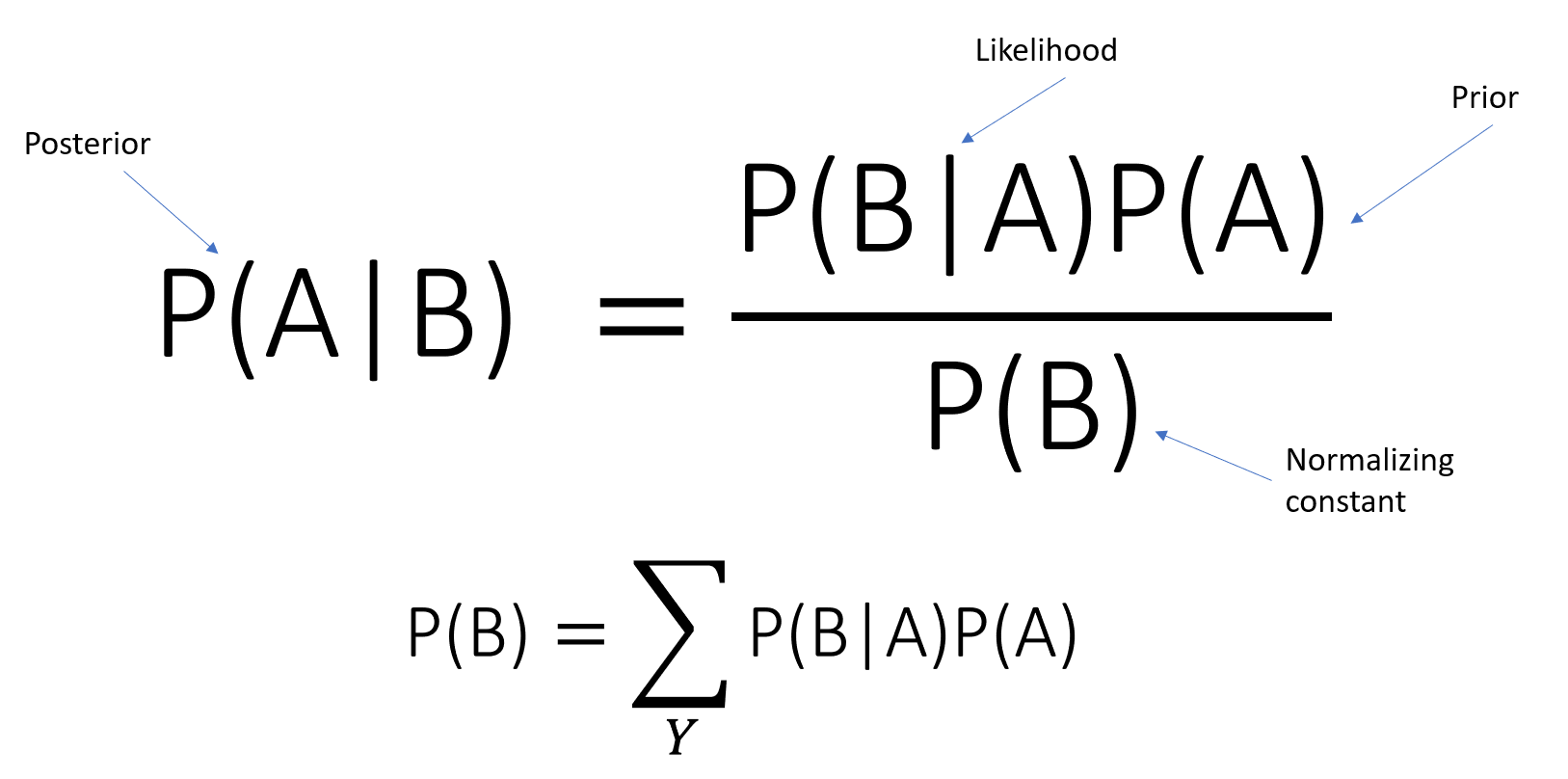
The theorem of Bayes gives us the probability that event A will occur since event B has occurred. For instance,

Given gloomy weather, what is the chance that it will rain? It is possible to call the possibility of rain as our hypothesis and to call the event reflecting cloudy weather as evidence.

As a posterior likelihood, P(A|B) is labeled
P(B|A)-is the conditional likelihood of B given A.
P(A)-is defined as the preceding likelihood of event A.
P(B) irrespective of the hypothesis

How Does the Naïve Bayes Classifier Work?

To demonstrate how the Naïve Bayes classifier works, we will consider an Email Spam Classification problem which classifies whether an Email is a SPAM or NOT.

Let’s consider we have total 12 emails. 8 of which are NOT-SPAM and remaining 4 are SPAM.

• Number of NOT-SPAM emails – 8
• Number of SPAM emails – 4
• Total Emails – 12
• Therefore, P(NOT-SPAM) = 8/12 = 0.666 , P(SPAM) = 4/12 = 0.333

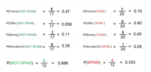
Suppose that only four terms [Friend, Bid, Money, Wonderful] constitute the entire Corpus. In each type, the following histogram represents the word count of each word.

Now we’ll measure each word’s conditional probabilities.

The below formula will measure the likelihood of the word Friend occurring as the mail is NOT-SPAM.

Calculating the probabilities for the whole text corpus.

We may apply the Bayes theorem to it, now that we have both the prior and conditional probabilities.

Suppose we get an email: “Offer Money” and we need to categorize it as SPAM or NOT-SPAM based on our previously determined probabilities.

Types of Naïve Bayes Classifier:

• Multinomial – It is used for Discrete Counts. The one we described in the example above is an example of Multinomial Type Naïve Bayes.
• Gaussian – This type of Naïve Bayes classifier assumes the data to follow a Normal Distribution.
• Bernoulli – This type of Classifier is useful when our feature vectors are Binary.

Implementation

Let’s import the required libraries:

#Loading the Dataset
from sklearn.datasets import load_breast_cancer
 
data_loaded = load_breast_cancer()
X = data_loaded.data
y = data_loaded.target

Then we fit training data to our model:

#Splitting the dataset into training and testing variables
from sklearn.model_selection import train_test_split
 
X_train, X_test, y_train, y_test = train_test_split(data.data, data.target, test_size=0.2,random_state=20)
 
#keeping 80% as training data and 20% as testing data.

The feature data (X-train) and the target variables are required as input arguments(y-train) by the .fit method of the GaussianNB class.

Now, let’s find out how accurate the accuracy metrics were used in our model.

#Import metrics class from sklearn
from sklearn import metrics
 
metrics.accuracy_score(y_predicted , y_test)

Accuracy = 0.956140350877193

We got accuracy around 95.61 %

Feel free to experiment with the code. You can apply various transformations to the data prior to fitting the algorithm.

What are Decision trees ?

The Decision Tree is a machine learning algorithm that uses a decision model and provides an event’s outcome/prediction in terms of chances or probabilities.
It is a non-parametric and predictive algorithm that provides the result on the basis of modeling those decisions/rules framed by observing the data characteristics.
Decision Trees learn from historic data as a supervised Machine Learning algorithm.

So, based on it, the algorithm trains and constructs the model of decisions, and then predicts the result.
Decision Trees can fulfill any of the following tasks:

• Record classification on the basis of probabilities to which group the records belong.
• A quality estimate of a certain target value.

In the upcoming segment, we will learn more about the above tasks.
A Decision Tree represents a structure resembling a flowchart that delivers the result based on probabilistic circumstances.

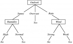
• The internal node for the attributes/variables represents the state.
• The outcome value of the condition is expressed by any branch.
• After resolving all the conditions of each attribute, the leaf nodes provide details about the decision to be made.

Different algorithms such as ID3, CART, C5.0, etc. are used by Decision Tree to determine the best attribute to be put as the root node value, which implies the best homogeneous set of data variables.

It starts with the comparison of the root node and the tree attributes. The comparison value tests the decision model. This continues until the expected outcome classification or estimation value hits the leaf node.
Now, let us take a look in-depth at the various forms of Decision Trees.

Types of DTrees

The following types of values are predicted by the Decision Tree:

• Classification: for the categorical data variables it predicts the class of the target value. Prediction, for instance, if the attribute gives the outcome as YES or NO.
• Regression: For numeric/continuous variables, it estimates the outcome value of the target variable. Prediction of the Bike Rental Count in the near time, for instance.

Assumptions 

• The whole training dataset is assumed as the value for the root node before the first iteration, i.e. before the model of decisions is specified.
• The values/attributes of the data are recursively distributed.
• It is believed that a mathematical approach is used to finalize the order in which the attribute is put as root/attribute node values.

Let’s implement

Having understood the working of Decision Trees, let us now implement the same in Python.

Let’s import the important libraries:

import os
import pandas as pd
import numpy as np
from sklearn.model_selection import train_test_split 
import numpy as np
from sklearn.tree import DecisionTreeRegressor

We have now specified a function to judge the error value of the Decision Tree’s output.

For this algorithm, we have used MAPE error metrics as this is an issue with regression evaluation.

def MAPE(Y_actual,Y_Predicted):
    Mape = np.mean(np.abs((Y_actual - Y_Predicted)/Y_actual))*100
    return Mape

We segregate the dataset into two data sets consisting of independent and dependent variables, moving it forward. In addition, we use the train-test-split() function to split the dataset into data training and testing.

bike = pd.read_csv("Bike.csv")
X = bike.drop(['cnt'],axis=1) 
Y = bike['cnt']
# Splitting the dataset into 80% training data and 20% testing data.
X_train, X_test, Y_train, Y_test = train_test_split(X, Y, test_size=.20, random_state=0)

Now is the time for the decision tree algorithm to be implemented. To build and train the model, we used the DecisionTreeRegressor() function.

In addition, using the predict() function, we predict the values of the target variable in the testing dataset.

After this, to get the accuracy of the model, we calculate the MAPE value (error value) and deduct it from 100.

DT_model = DecisionTreeRegressor(max_depth=5).fit(X_train,Y_train)
DT_predict = DT_model.predict(X_test) #Predictions on Testing data
DT_MAPE = MAPE(Y_test,DT_predict)
Accuracy_DT = 100 - DT_MAPE
print("MAPE: ",DT_MAPE)
print('Accuracy of Decision Tree model: {:0.2f}%.'.format(Accuracy_DT))
print("Predicted values:\n",DT_predict)

Output:

MAPE:  18.076637888252062Accuracy of Decision Tree model: 81.92%.Predicted values:[3488.279069774623.467213112424.4623.467213114883.190476196795.117686.751728.121212122602.666666672755.173913044623.467213114623.467213111728.121212126795.115971.142857141249.524623.467213116795.113488.279069775971.142857143811.636363642424.1249.526795.116795.113936.343753978.51728.121212126795.111728.121212123488.279069776795.116795.115971.142857141728.121212124623.467213111249.523936.343753219.583333337686.754623.467213112679.56795.112755.173913046060.785714296795.114623.467213116795.116795.114623.467213114883.190476194623.467213112602.666666674623.467213117686.756795.117099.51728.121212126795.111249.524623.467213116795.114623.467213111728.121212124883.190476194623.467213116795.116795.114623.467213111728.121212124623.467213114623.467213111178.56795.114623.467213116795.116795.111728.121212123488.279069776795.115971.142857146060.785714294623.467213113936.343751249.521728.121212124676.333333333936.343754623.467213116795.114623.467213114623.467213116795.115971.142857144883.190476194883.190476193488.279069776795.116795.116795.113811.636363646795.116795.116060.785714294623.467213111728.121212124623.467213116795.116795.114623.467213111728.121212126795.111728.121212123219.583333331728.121212126795.111249.526795.112755.173913041728.121212126795.115971.142857141728.121212124623.467213114623.467213114676.333333336795.113936.343754883.190476193978.54623.467213114623.467213113488.279069776795.116795.113488.279069774623.467213113936.343752600.3488.279069772755.173913046795.114883.190476193488.27906977]