Hello, readers. Welcome to codegigs. If this is your first time on the site, I would suggest you to bookmark us. We provide detailed, explanatory articles for data science.
In this article, I’ll try to cover all the base knowledge you’ll need for getting started with OpenCV, and then we’ll do a project along the way. So let’s get started ->
Google colaboratory setup
First, we’ll be opening up Google colab, our trusted python notebook. Go to https://colab.research.google.com/ and sign in with your Google account.
Next, we’ll download a video from youtube for use.
Downloading videos from youtube
We’ll be installing a handy tool that I use a lot daily – YoutubeDL. The code for installing it is given below:
!sudo pip install --upgrade youtube_dl

!youtube-dl "https://www.youtube.com/watch?v=zN-FXGpVABQ"
This will download a funny cat video to your local colab environment!
Now let’s briefly go over the basics of OpenCV.
Basic knowhow of OpenCV
OpenCV stands for Open Source Computer Vision Library. It came out around 2000 and has seen a significant amount of support in the community.
(Even though we’ll be using python in this article, know that the same can be performed using any other programming language, so take your pick.)
OpenCV-Python is a library of Python bindings designed to solve computer vision problems.
Numpy, a highly efficient library for numerical operations with a MATLAB-style syntax, is used by OpenCV-Python.
Install OpenCV directly using pip :
pip3 install OpenCV-python
Now let’s work with an image first. You can use any. I used the
1. Simple matrix operations on images
The scaling of images is referred to as image resizing. Scaling is useful in a variety of image processing and machine learning applications. It aids in the reduction of the number of pixels in an image, which has various advantages, for example. It can reduce the time it takes to train a neural network since the more pixels in an image there are, the more input nodes there are, which raises the complexity.
Get the picture:
!wget -O "pic.jpg" "https://static2.srcdn.com/wordpress/wp-content/uploads/2020/07/Ash-Pikachu-Pokemon-Anime.jpg"
import cv2

image = cv2.imread("pic.jpg")

plt.imshow(image)

plt.show()
Gaussian = cv2.GaussianBlur(image,(5,5),2)

plt.imshow(Gaussian)

Median filtering is commonly employed in digital image processing because it preserves edges while reducing noise under specific conditions. It’s one of the most effective algorithms for eliminating salt and pepper noise.
median = cv2.medianBlur(image,1)

plt.imshow(median)
consider this image which is very noisy:
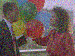
Now if we use median blur on it:
!wget -O "balloons.jpg" "https://people.sc.fsu.edu/~jburkardt/cpp_src/image_denoise/balloons_noisy.png"
image2 = cv2.imread("balloons.jpg")
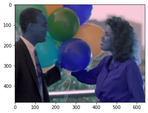
median = cv2.medianBlur(image2,5)
plt.imshow(median)
We can see that the image has been completely denoised!
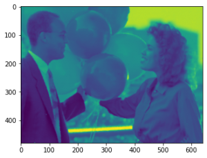
To convert this image into grayscale,
gray_image = cv2.cvtColor(median, cv2.COLOR_BGR2GRAY)

plt.imshow(gray_image)
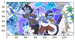
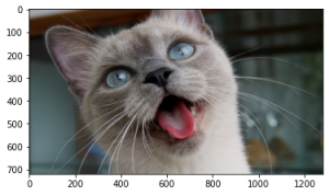
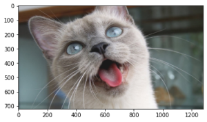
Let’s download another picture :
!wget -O "pic.jpg" "https://i.ytimg.com/vi/0cwNIwyXifw/maxresdefault.jpg"

image=cv2.imread('pic.jpg')

image=cv2.cvtColor(image, cv2.COLOR_BGR2RGB)

plt.imshow(image)
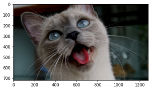
We know to grayscale the image:
gray_image=cv2.cvtColor(image,cv2.COLOR_BGR2GRAY)

plt.imshow(gray_image)
There are a few other modes, like hsv (hue, saturation, value):
hsv_image=cv2.cvtColor(image,cv2.COLOR_BGR2HSV)

plt.imshow(hsv_image)
We can type image[0,0] #This is the B,G,R values of the first pixel
We can create histograms of the BGR channels too!
We use the cv2.calcHist along with matplotlib.
import matplotlib.pyplot as plt
color = [‘b’,’g’,’r’]
#the enumerate is a built in function which gives you tuples of (index,list_element)
for i,col in enumerate(color):
hist=cv2.calcHist([image],[i],None,[256],[0,256])
plt.plot(hist,color=col)
plt.xlim([0,256])
plt.show()
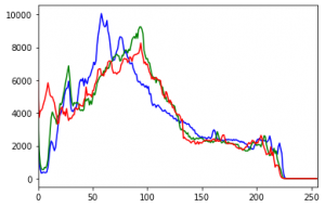
The calcHist function has 5 arguments:
1. [image] (even though it is already a matrix, we need to give another square bracket)
2. channel:
[0] = blue (for color images) / grayscale (for grayscale images)
[1] = green
[2] = red
3. mask: we can either create a mask/selection of the image (later),
or the value “None” gives us the full scale image
4. bin size: this is the bin size of the histogram.
[256] = full scale
5. range: generally [0,256]
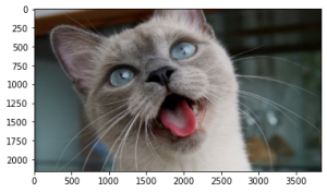
2. Scaling up
This is an important functionality that I feel we should learn –
image_scaled_by_fourth=cv2.resize(image,None,fx=0.25,fy=0.25)
# arguments are: (image, dimensions of output(width,height), x_scale, y_scale)

While the above code gives us a 1/4th image, we can increase the size of an image by interpolation techniques.
To scale it up, we can use any of these 5 interpolation techniques:
1. INTER_AREA
2. INTER_NEAREST
3. INTER_LINEAR
4. INTER_CUBIC
5. INTER_LANCZOS4
image_zoom_2 = cv2.resize(image,None,fx=3,fy=3,interpolation=cv2.INTER_LANCZOS4)

plt.imshow(image_zoom_2)
Another method to quickly scale images is using the inbuilt pyramid functions: pyrDown pyrUp, which are relatively easier and less technical.
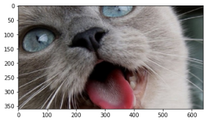
3. Crop and Brighten/Darken images
There is no inbuilt function to crop images. BUT we can use NumPy slicing on the image matrix!
h,w = image.shape[:2]

cropped = image[int(h*.25):int(h*.75),int(w*.25):int(w*.75)]

plt.imshow(cropped)
We can also brighten or darken images:
M=np.ones(image.shape,"uint8")

added=cv2.add(image,M*25)

subtracted=cv2.subtract(image,M*25)

plt.imshow(added)

plt.imshow(subtracted)
Text manipulation
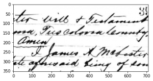
This is used to bring more clarity to the text and is widely used on handwritten text.
Consider this image:
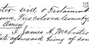
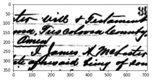
Now we can make this font bolder using the technique called erosion:
text=cv2.imread("text.jpg")

# Creating kernel

kernel = np.ones((5, 5), np.uint8)

# Using cv2.erode() method

eroded = cv2.erode(text, kernel)

dilated = cv2.dilate(eroded, kernel)
That’s all for this article. I’ve hopefully provided enough techniques for you to practice. Until next time!
Time taken for the execution of all commands in this article:
10 loops, best of 5: 184 ms per loop
— Arkaprabha-Majumdar —