Why Plotly?

Plotly’s Python graphing library is an interactive, open-source plotting library that supports over 40 unique chart types. These chart types cover a wide range of statistical, financial, geographic, scientific, and 3-dimensional use-cases. We will walk through how to make interactive, publication-quality graphs ranging from line plots, scatter plots, to histograms, heatmaps, subplots, and bubble charts. Let’s compare Plotly with Matplotlib, another commonly used library for data visualization in data science. We will create synthetic data and then plot data with both Matplotlib and Plotly.

Importing required libraries:

import pandas as pd
import numpy as np
import matplotlib.pyplot as plt 
import plotly.offline as pyo

Creating a matplotlib plot:

# create fake data:
df = pd.DataFrame(np.random.randn(100,4),columns=['col1','col2','col3','col4'])
df.plot()
plt.show()

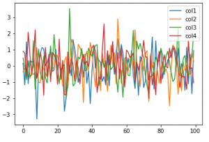
This is just a static image without any interactivity.

Creating a plotly plot:

pyo.plot([{
'x': df.index,
'y': df[col],
'name': col
} for col in df.columns])

 

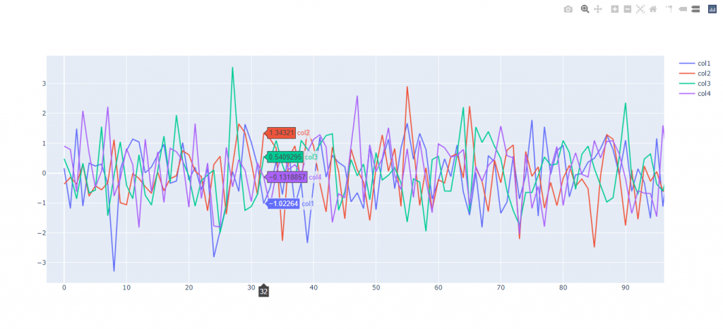
1. You can compare data while hovering over the plot as shown in figure above.
2. Clicking on a trace on legend hides it and double-clicking a trace isolates it. Double-click again to redisplay the other traces.
3. A file named temp-plot.html is saved in your working directory (i.e. where your .py file is saved). We’ll see later how adding a filename=’something-else.html’ argument lets you change the name of the file (useful when working with multiple plots). Re-running .py or jupyter notebook replaces earlier copies of the file.
4. You can also download this plot to a static .png image file if you want.

Creating Scatter plots with Plotly:

import plotly.offline as pyo
import plotly.graph_objs as go
import numpy as np
np.random.seed(42)
random_x = np.random.randint(1,101,100)
random_y = np.random.randint(1,101,100)
data = [go.Scatter(
    x = random_x,
    y = random_y,
    mode = 'markers',
    marker = dict( # change the marker style
        size = 12,
        color = 'rgb(51,204,153)',
        symbol = 'pentagon',
        line = dict(
        width = 2,
        )
    )
)]
layout = go.Layout(
    title = 'Random Data Scatterplot', # Graph title
    xaxis = dict(title = 'Some random x-values'), # x-axis label
    yaxis = dict(title = 'Some random y-values'), # y-axis label
    hovermode ='closest') # handles multiple points landing on the same vertical
fig = go.Figure(data=data, layout=layout)
pyo.plot(fig, filename='scatter_plot.html')

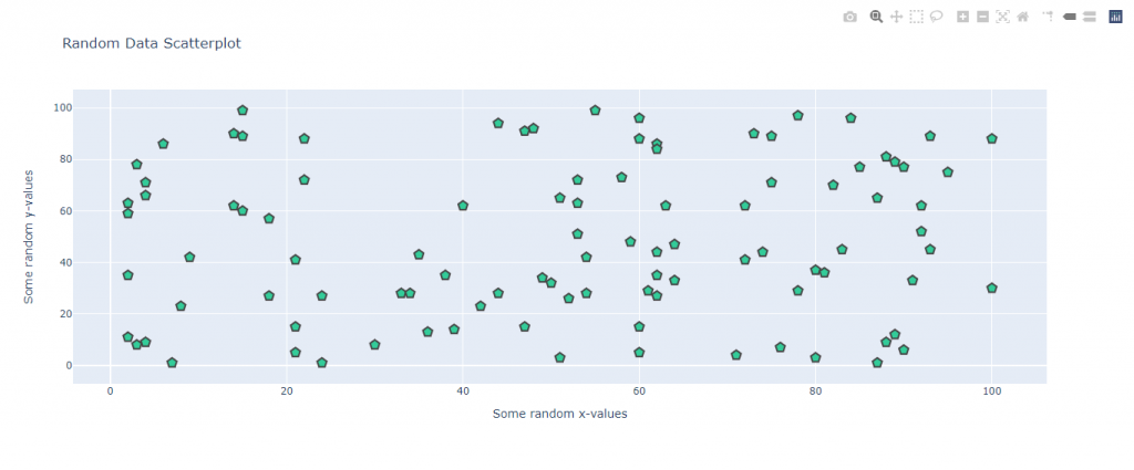
Notice how we bundled both the data and the layout inside a Figure , and had plotly graph the figure as HTML. We also used following argument to change the marker style:

marker = dict( # change the marker style
        size = 12,
        color = 'rgb(51,204,153)',
        symbol = 'pentagon',
        line = dict(
        width = 2,
        )

Bubble Charts

Bubble charts simply scatter plots with the added feature that the size of the marker can be set by the data.

Changing the above code for ‘markers’ with the given below will give us a bubble chart. Try it out yourself!

marker = dict( # change the marker style
        size = 1.5*random_x,
        color = 'rgb(51,204,153)',
        line = dict(
        width = 2,
        )

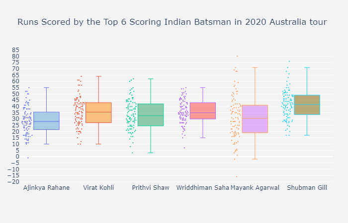
Creating Box plots with Plotly:

At times it’s important to determine if two samples of data belong to the same population. Box plots are great for this! The shape of a box plot (also called a box-and-whisker-plot) doesn’t depend on aggregations like sample mean. Rather, the plot represents the true shape of the data. Also, depending on how the whiskers are constructed, box plots are useful for identifying true outliers of a data set. A box plot identifies those points that lie far from the median compared to the rest of the data. A boxplot is constructed of two parts, a box and a set of whiskers shown in Figure 2. The lowest point is the minimum of the data set and the highest point is the maximum of the data set. The box is drawn from Q1 to Q3 with a horizontal line drawn in the middle to denote the median where Q1 and Q3 are first and third quartile respectively.

import plotly.graph_objects as go
import numpy as np

x_data = ['Ajinkya Rahane', 'Virat Kohli',
          'Prithvi Shaw', 'Wriddhiman Saha',
          'Mayank Agarwal', 'Shubman Gill',]

N = 100

y0 = (10 * np.random.randn(N) + 30).astype(np.int)
y1 = (13 * np.random.randn(N) + 38).astype(np.int)
y2 = (11 * np.random.randn(N) + 33).astype(np.int)
y3 = (9 * np.random.randn(N) + 36).astype(np.int)
y4 = (15 * np.random.randn(N) + 31).astype(np.int)
y5 = (12 * np.random.randn(N) + 40).astype(np.int)

y_data = [y0, y1, y2, y3, y4, y5]

colors = ['rgba(93, 164, 214, 0.5)', 'rgba(255, 144, 14, 0.5)', 'rgba(44, 160, 101, 0.5)',
          'rgba(255, 65, 54, 0.5)', 'rgba(207, 114, 255, 0.5)', 'rgba(127, 96, 0, 0.5)']

fig = go.Figure()

for xd, yd, cls in zip(x_data, y_data, colors): #some data manipulation to add a trace to our figure like earlier
        fig.add_trace(go.Box(
            y=yd,
            name=xd,
            boxpoints='all',
            jitter=0.5,
            whiskerwidth=0.2,
            fillcolor=cls,
            marker_size=2,
            line_width=1)
        )

fig.update_layout(
    title='Runs Scored by the Top 9 Scoring Indian Batsman in 2020 Australia tour',
    yaxis=dict(
        autorange=True,
        showgrid=True,
        zeroline=True,
        dtick=5,
        gridcolor='rgb(255, 255, 255)',
        gridwidth=1,
        zerolinecolor='rgb(255, 255, 255)',
        zerolinewidth=2,
    ),
    margin=dict(
        l=40,
        r=30,
        b=80,
        t=100,
    ),
    paper_bgcolor='rgb(243, 243, 243)',
    plot_bgcolor='rgb(243, 243, 243)',
    showlegend=False
)

fig.show()

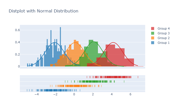
Creating Dist plots with Plotly:

Distribution Plots, or Displots, typically layer three plots on top of one another. The first is a histogram, where each data point is placed inside a bin of similar values. The second is a rug plot – marks are placed along the x-axis for every data point, which lets you see the distribution of values inside each bin. Lastly, Displots often include a “kernel density estimate”, or KDE line that tries to describes the shape of the distribution.

import plotly.figure_factory as ff
import numpy as np

# Add histogram data
x1 = np.random.randn(200)-2
x2 = np.random.randn(200)
x3 = np.random.randn(200)+2
x4 = np.random.randn(200)+4

# Group data together
hist_data = [x1, x2, x3, x4]

group_labels = ['Group 1', 'Group 2', 'Group 3', 'Group 4']

# Create distplot with custom bin_size
fig = ff.create_distplot(hist_data, group_labels,curve_type='normal', bin_size=[.1, .25, .5, 1])
# Add title
fig.update_layout(title_text='Distplot with Normal Distribution')
fig.show()

These were a few examples of how to use Plotly to create amazing plots and charts. In the next post, we will go through the basics of Dash which will enable you to design and build a basic dashboard from scratch in Python.